Time Series Analysis for Financial Forecasting

directional trends, repeating seasonal cycles, and irregular fluctuations. The trend component might show a company's revenue growing 5% annually, while seasonality could reveal quarterly spikes around holidays. Random variations then overlay these predictable elements.

Seasonality often follows natural rhythms - retail sales peaking in December or tourism rising each summer. These patterns persist until underlying conditions change, making them invaluable for planning. Meanwhile, multi-year business cycles reflect broader economic forces that require different analytical approaches than fixed-interval seasonality.

Methods for Time Series Analysis

Visual exploration provides the first analytical layer. Simple line graphs can reveal obvious patterns, while decomposition plots separate trend, seasonal, and residual components. Statistical tests then quantify these observations - the Augmented Dickey-Fuller test checks for stationarity, while autocorrelation functions map dependency structures.

Modern analysis blends classical and machine learning approaches. ARIMA models excel with linear relationships, while LSTM neural networks capture complex nonlinear patterns. The key lies in matching method to data characteristics - some series respond well to simple exponential smoothing, while others demand sophisticated hybrid models.

Applications of Time Series Analysis

Financial markets represent the classic application, where analysts predict asset prices and volatility. Economic forecasting uses similar methods to project GDP, unemployment, and inflation. Less obviously, hospitals apply these techniques to predict patient admissions, while manufacturers optimize inventory against anticipated demand.

The true power emerges when time series analysis informs real decisions. A retailer might adjust staffing and inventory based on seasonal forecasts, while an investor could time market entries using volatility predictions. These applications demonstrate how temporal patterns translate into competitive advantage.

Key Concepts in Time Series Analysis

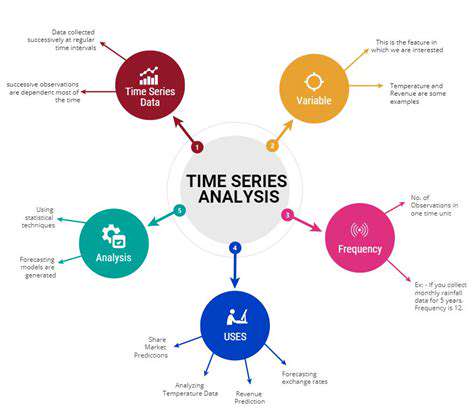
Understanding Time Series Data

Time-ordered data creates unique analytical opportunities and challenges. The sequence itself contains information - stock prices form patterns, economic indicators follow leading/lagging relationships, and sensor data shows system dynamics. Temporal context transforms independent data points into a connected story.

Effective analysis begins with domain understanding. Are weekends excluded from this sales data? Does daylight saving time affect these measurements? Such contextual knowledge ensures proper interpretation of observed patterns and prevents analytical missteps.

Stationarity and its Importance

Stationary series maintain consistent statistical properties - constant mean, variance, and autocorrelation - across time segments. Many models require this stability for reliable predictions. Economic shocks or regime changes often violate stationarity assumptions, requiring transformations.

Differencing - subtracting consecutive values - frequently converts non-stationary data into stationary form. Other approaches include logarithmic transformations or structural break adjustments. The Phillips-Perron and KPSS tests complement the Dickey-Fuller approach for robust stationarity assessment.

Trend Analysis

Trend extraction separates persistent movements from short-term fluctuations. A linear trend might suffice for steady growth, while piecewise regression can capture changing growth rates. The Hodrick-Prescott filter offers another approach, separating cyclical from trend components.

Misidentified trends distort all subsequent analysis. An apparent upward trend might actually reflect structural breaks or level shifts. Multivariate approaches can help distinguish true trends from confounding factors.

Seasonality and Cyclical Components

Seasonal decomposition (e.g., STL) quantifies regular intra-year patterns, while Fourier analysis identifies underlying periodicities. Proper seasonal adjustment reveals underlying trends - crucial for month-to-month retail performance comparisons.

Cycles lack fixed periods, requiring different detection methods. Spectral analysis identifies dominant frequencies, while wavelets localize cyclical patterns in time. Business cycle analysis often combines multiple indicators to identify expansion and contraction phases.

Model Selection and Evaluation

The model zoo includes ARIMA, GARCH for volatility, VAR for multivariate systems, and newer machine learning hybrids. Selection depends on data characteristics and forecast horizon. Short-term predictions might use simple models, while long-range forecasts benefit from incorporating external variables.

Backtesting against historical data validates model robustness. Walk-forward validation tests how models would have performed in real-time forecasting, exposing overfitting. Information criteria (AIC/BIC) balance fit quality against model complexity.

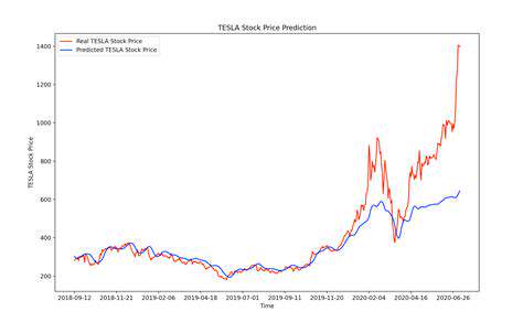
Applying Time Series Models in Financial Forecasting

Understanding Time Series Data in Finance

Financial markets generate complex time series reflecting countless transactions and decisions. Prices incorporate expectations, creating challenging forecasting problems. Returns typically show volatility clustering - calm and turbulent periods - while volumes may exhibit different seasonal patterns than prices.

The efficient market hypothesis suggests prices reflect available information, making pure time series prediction difficult. However, anomalies like momentum and mean-reversion effects create opportunities. Successful models often combine time series techniques with cross-asset relationships and macroeconomic factors.

Applying Various Time Series Models

Simple models provide benchmarks. Random walks often outperform complex models for liquid assets, demonstrating forecasting difficulties. Moving averages underpin many technical trading strategies, while exponential smoothing adapts flexibly to recent changes.

GARCH models excel in volatility forecasting, crucial for risk management. For multivariate problems, vector autoregression (VAR) captures inter-asset dynamics. The most sophisticated approaches combine these statistical methods with machine learning for enhanced pattern recognition.

Regardless of methodology, robust financial forecasting requires continuous model monitoring. Structural breaks occur during crises, and changing market regimes demand model adjustments. The best practitioners blend quantitative models with qualitative judgment about market conditions.